Embarrassingly Parallel Reduction in CUDA
Published:
When life gives you arrays, reduce them. Aggresively.
Reduce operations are common in HPC applications. Put simply, a reduce operation combines all elements of an array into a single value through either sum, min, max, product, etc.
Reduce operations are embarrasingly parallel1, which makes them a great candidate to be run on GPUs.
This post will walk through a series of optimizations to iteratively obtain maximum device throughput.
Code is available on GitHub.
| # | Kernel | Bandwidth (GB/s) | Relative to jnp.sum |
|---|---|---|---|
| 1 | Vector Loads | 9.9 | 1.1% |
| 2 | Tree Reduction | 223 | 24.7% |
| 3 | Non-divergent Threads | 317 | 36.3% |
| 4 | Sequential Addressing | 331 | 38.0% |
| 5 | Reduce on First Load | 618 | 70.9% |
| 6 | Warp Unrolling | 859 | 98.6% |
| 0 | jnp.sum reference | 871 | 100% |
Roofline
Our bench problem is to compute the sum of elements of a vector with \(N = 2^{25}\) floats. A reduce operation reads each element of the array at least once. And because this is a sum operation, it will also do a total of \(N-1\) adds. First, we will lower-bound our runtime based on peak compute and memory throughput values of an RTX-30902:
- \(N\)
float32reads at 936 GB/s = 0.136 ms - \(N-1\)
float32adds at 35.6 TFLOPS = 0.0036 ms
As we can see, reduction operations have very low arithmetic intensity, they are memory-bound.
The theoretical minimum time for this operation is 0.136 + 0.0036 = 0.1396 ms. Since CUDA does not provide a built-in reduce_sum primitive, we will use jax.numpy.sum as a reference. jnp.sum completes in 0.15 ms, achieving 871 GB/s effective bandwidth.
Complexity Analysis
Brent’s theorem is how we compare efficiency across different parallel algorithms. For a parallel algorithm, we can calculate:
- \(W\): work, the total number of operations if run serially.
- \(S\): step complexity, or the serialization cost when certain operations cannot be parallelized.
- \(P\): number of parallel processors.
Given this, time complexity with \(P\) parallel processors is defined as:
\[\begin{equation} T_p \le \frac{W}{P} + S \end{equation}\]We can derive a couple of interesting bounds which will be helpful later:
- \(T_\infty = S\): Infinite parallelism boils down to the time taken in sequential operations.
- \(T_1 = W\): Single processor time is when the total work is performed sequentially.
- \(T_1 / T_p\): Speedup when using \(P\) processors.
- \(W / S\): Parallelism achievable in the algorithm.
For the reduce_sum operation, work complexity \(W = N_{reads} + (N-1)_{adds}\) is \(O(N)\).
Baseline
Jensen would hate me for using GPUs to sum \(N\) elements using atomic operations. But this “serial” operation serves as a baseline for all parallelism we will achieve later.
__global__ void reduce_sum_kernel1(float *out, const float *arr, int N) {
  int idx = blockIdx.x * blockDim.x + threadIdx.x;

  if (idx < N) {
    atomicAdd(out, arr[idx]);
  }
}
This kernel achieves 2.47 GB/s effective bandwidth.
Kernel 1: Vector Loads
We will start with a naive optimization. We let each thread compute a portion of the array sum in parallel, and accumulate the partial sums to the output. Since our GPU supports 128-byte load/stores, we will use the float4 vector data type.
Here is what the computation looks like for an array with \(N = 16\) elements:
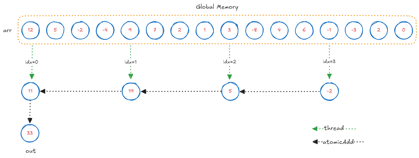
__global__ void reduce_sum_kernel1(float *out, const float4 *arr, int N) {
  int idx = blockIdx.x * blockDim.x + threadIdx.x;

  if (idx < N) {
    float4 val = arr[idx];
    atomicAdd(out, val.x + val.y + val.z + val.w);
  }
}
Technicaly, this kernel could even saturate the memory bus using \(k\)-wide vector loads and \(k\) sums per thread. We achieve 9.9 GB/s effective bandwidth with \(k=4\): a \(4\times\) throughput.
Let’s not be fooled here. This is actually not a parallel algorithm.
Complexity analysis:
Work complexity \(W\) of this kernel is \(O(N)\) - all elements of the array are accessed and summed once. This is the minimum work required even for a serial algorithm. Therefore, this kernel is work efficient.
Step complexity \(S\) for this kernel is \(O(N/4) \approx O(N)\) - as all \(N/4\) threads must wait for the
atomicAddto complete. This kernel is not step efficient.Parallelism ratio \(\frac{W}{S} = \frac{O(N)}{O(N)} = 1\). This means the kernel does not scale with processors. In other words: even if we had infinite processors with infinite memory bandwidth, this kernel behaves serially under
atomicAddoperations.
An algorithm is parallelizable if \(\frac{W}{S} > 1\). Can we compute sum in less than \(N\) steps?
Kernel 2: Tree Reduction
The problem with the previous kernel is that it was not step efficient. It takes \(O(N)\) steps to sum over the array. Using a binary tree reduction, we can sum the array in \(\log N\) steps. Note that we still do \(N-1\) adds and \(N\) reads. Therefore this approach remains work efficient.
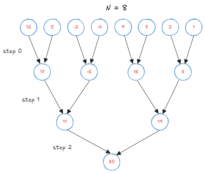
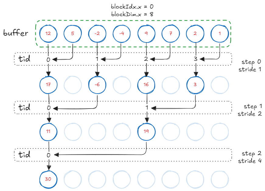
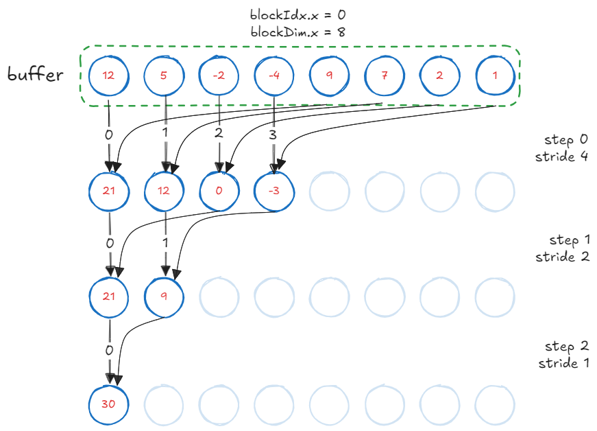
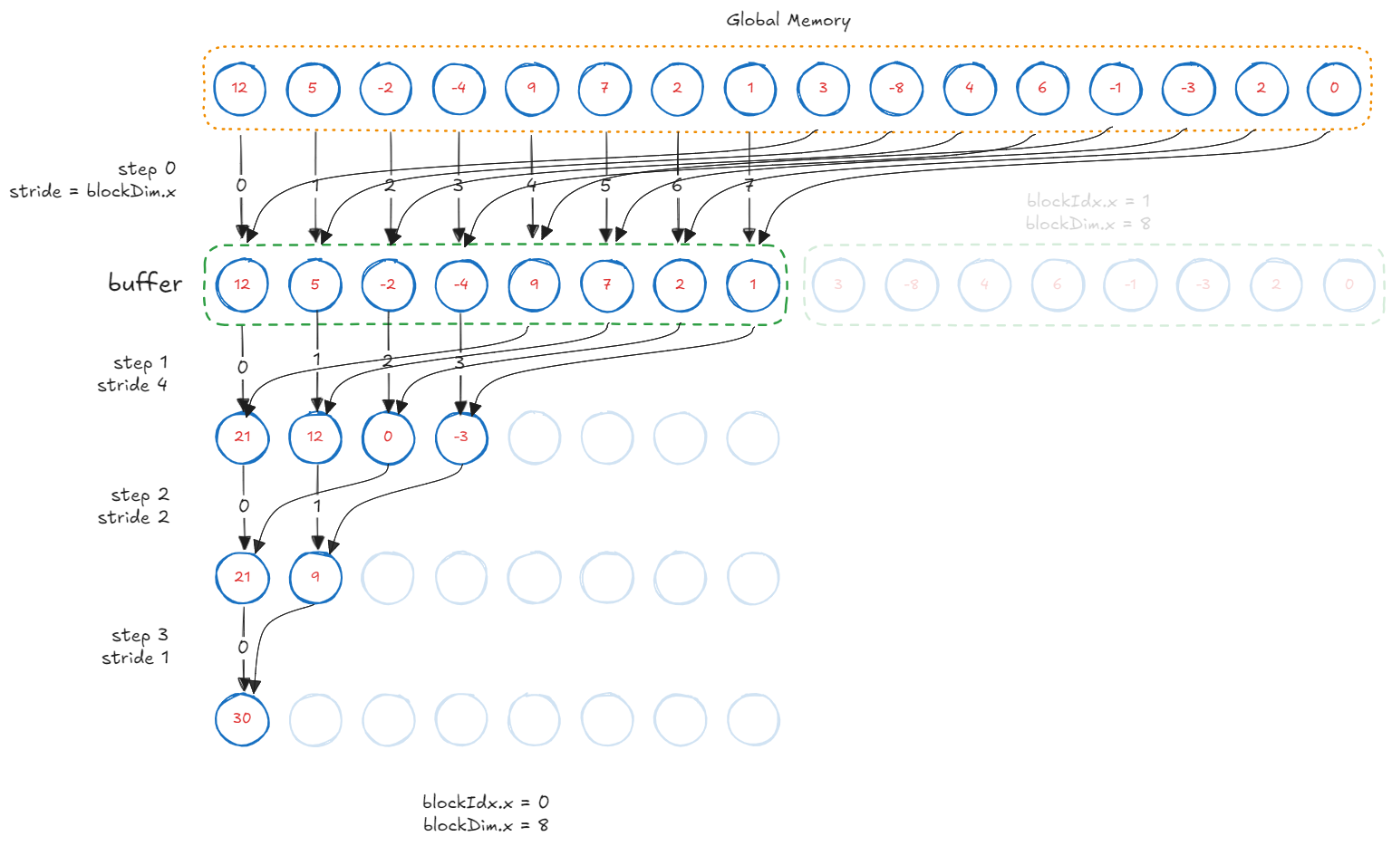
In CUDA, threads are grouped as “blocks”. We will divide the array into blocks of certain size, which is a tunable parameter. Each block will sum its elements in parallel, and then the partial sums will be accumulated using atomics. For simplicity, I will depict the reduction process for a block_size of 8.
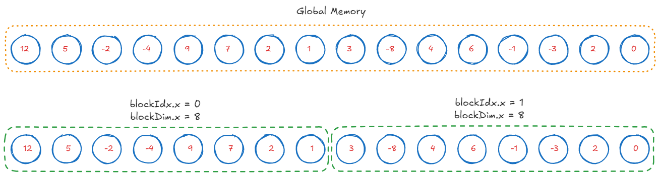
We load subarrays of size block_size into shared memory. We will use this buffer to store the partial sums.
// a buffer that can hold 8 floats
extern __shared__ float buffer[];

/**
 * blockDim.x = 8, number of threads per block
 * blockIdx.x = 0 or 1, id of the block
 * threadIdx.x = 0...7, id of the thread within the block
 */
int idx = blockIdx.x * blockDim.x + threadIdx.x;

// thread idx within the block, 0...7
int tid = threadIdx.x;

// Load a tile
buffer[tid] = arr[idx];

// Don't proceed until all threads have loaded their values
__syncthreads();
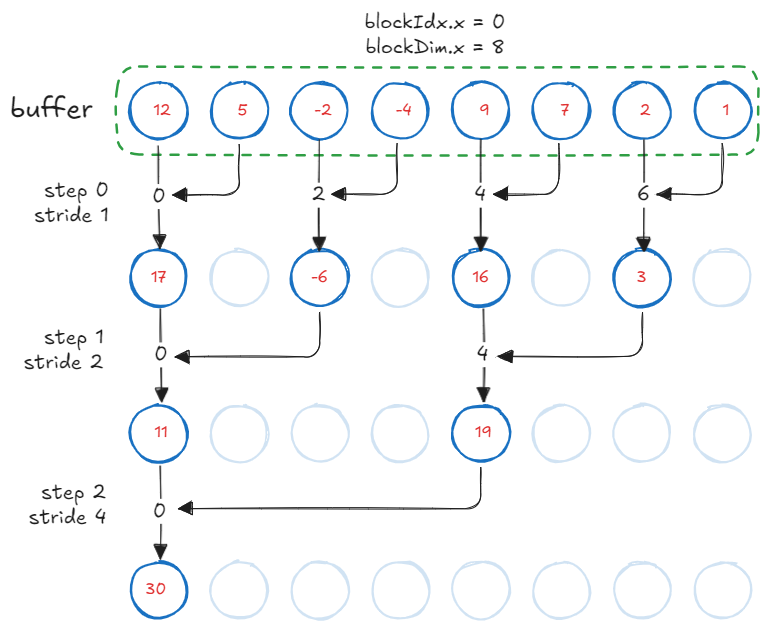
We perform the reduction once the buffer is populated. GPU invokes all blocks in parallel. Each block performs a tree reduction on the buffer. The process is as follows:
- At the first step, consecutive elements are summed by
tid=[0, 2, 4, 6]. - At the second step, every second element gets summed by every second thread
tid=[0, 4]. - This process continues until the final sum is stored in
buffer[0].
After \(\log N\) reductions, each block performs an atomicAdd to the output. Note that this kernel always performs as many atomicAdd operations as there are number of blocks executing in parallel. Unlike our vector-load kernel, the number of atomic operations here is not dependent on the array size.
__global__ void reduce_sum_kernel1(float *out, const float *arr, int N) {
  extern __shared__ float buffer[];
  int idx = blockIdx.x * blockDim.x + threadIdx.x;
  int tid = threadIdx.x;

  if (idx < N) {
    buffer[tid] = arr[idx];
    __syncthreads();

    for (int s = 1; s < blockDim.x; s *= 2) {
      if (tid % (2 * s) == 0) {
        buffer[tid] += buffer[tid + s];
      }
      __syncthreads();
    }

    if (tid == 0) {
      atomicAdd(out, buffer[0]);
    }
  }
}
This kernel achieves 223 GB/s effective bandwidth, a \(23\times\) improvement.
Complexity analysis:
- Work complexity \(W\) of this kernel is \(O(N)\). Therefore, this kernel is work efficient.
- Step complexity \(S\) for this kernel is \(O(\log N)\). Therefore, this kernel is step efficient.
- Parallelism ratio \(\frac{W}{S} = \frac{O(N)}{O(\log N)} = O(N/\log N)\) is greater than 1. This is our first truly parallel algorithm.
Kernel 3: Non-divergent Threads
Now that we have an algorithm that is both work and step efficient, all further improvements will be a result of specializing memory and computation patterns for the actual hardware.
The previous kernel suffers from two issues:
Warp divergence: Odd numbered threads remain unused. On CUDA devices, threads within a block are organized in groups of
32, called warps. When threads of a warp “branch”, the warp is said to be divergent. Compiler serializes these branches.Modulo arithmetic: At each step, half the active threads enter the
ifblock, perform expensive arithmetic while not participating in the computation.
// Only evenly strided threads are active, plus % is wasteful.
if (tid % (2 * s) == 0) {
    buffer[tid] += buffer[tid + s];
}
We eliminate % operation and compute an index such that only consecutive threads in a block are active. The inner loop now becomes:
int index = 2 * s * tid;
if (index < blockDim.x) {
    buffer[index] += buffer[index + s];
}
With this change, our kernel achieves 317 GB/s effective bandwidth, a 42% improvement over the previous kernel.
Bank Conflicts3
On CUDA devices, shared memory is divided into groups of 32 banks, assuming each index holds 4-byte wide memory (called a word). Bank ID relates to the index of memory being accessed as follows:
If different threads access different banks in parallel, shared memory can serve all those requests with no penalty. However, if two threads access indices from the same bank at the same time, the memory controller serializes these requests. These are called bank conflicts. Below is an example of a two-way bank conflict when different threads wrap around the same bank index: buffer[threadIdx.x * 2]
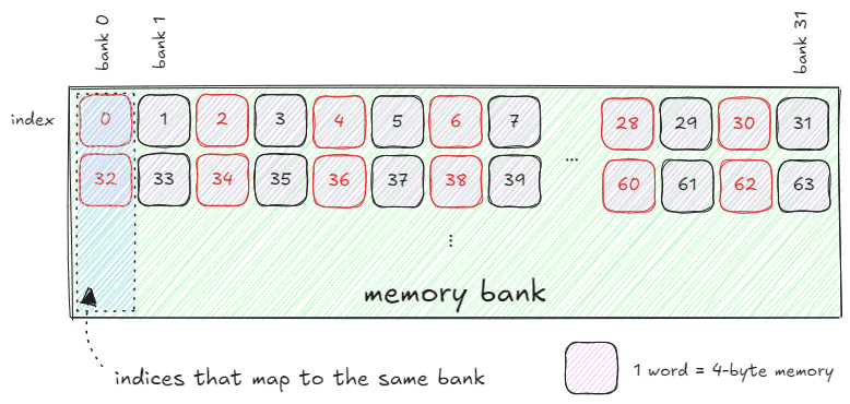
For instance, with our non-divergent threads kernel:
- At stride
s=1,tid=[0,16]accessindex=[0,32]andindex[1,33]which belong to the same bank. - At stride
s=2,tid=[0,8]accessindex=[0,32]andindex[2,34]which belong to the same bank. and so on.
In summary, when different threads start accessing addresses that wrap around the bank index (due to modulo 32 behavior), it may lead to 2-way, 4-way, or even higher-degree conflicts. We will see how to eliminate bank conflicts in the next kernel.
Kernel 4: Sequential Addressing
There is one neat trick up CUDA’s sleeves. It is not a bank conflict if the same thread accesses multiple addresses within the same bank. Looking at the conflict example, we want tid=0 to access index=[0,32], tid=1 to access index=[1,33] and so on. To do so, we invert the stride calculation.
// halve stride on each step
for (int s = blockDim.x / 2; s > 0; s /= 2) {

  // bounds checking
  if (tid < s) {
    buffer[tid] += buffer[tid + s];
  }
  __syncthreads();
}
This kernel achieves 335 GB/s effective bandwidth. While this change might not seem as impressive in terms of speedup, sequential addressing and elimination of bank conflicts is the foundation for our next banger.
Kernel 5: Reduce on First Load
Half the threads in each block do not perform any computation during the first reduction step. We can halve the total blocks and let each thread perform first level of reduction while loading elements in the buffer.
buffer[tid] = arr[idx] + arr[idx + blockDim.x];
This kernel achieves 618 GB/s effective bandwidth, over 1.86 \(\times\) faster.
Kernel 6: Warp Unrolling
Sequential addressing has a key feature: threads that finish execution become idle for the rest of the program. When number of active threads become less than 32, all these threads are part of the same “warp” in their respective blocks. Threads that are part of the same warp do not need thread synchronization calls or bounds checking. This reduces instruction overhead.
By unrolling the reduction for last 32 elements, we eliminate useless work in all warps of all blocks.
// Reduce synchronously across blocks until we have 32 threads left.
for (int s = blockDim.x / 2; s > 32; s /= 2) {
  if (tid < s) {
    buffer[tid] += buffer[tid + s];
  }
  __syncthreads();
}

// Unroll and reduce for the last 32 threads.
if (tid < 32) {
  warpReduce(buffer, tid);
}
We define a device function to unroll the warp and perform reductions.
__device__ void warpReduce(volatile float *buffer, int tid) {
  buffer[tid] += buffer[tid + 32];
  buffer[tid] += buffer[tid + 16];
  buffer[tid] += buffer[tid + 8];
  buffer[tid] += buffer[tid + 4];
  buffer[tid] += buffer[tid + 2];
  buffer[tid] += buffer[tid + 1];
}
We are now at 859 GB/s effective bandwidth, within ~1% of jax.numpy.sum.
Who doesn’t like speed?