The Blessing of Dimensionality

Grant recently published a video on how certain geometry puzzles become trivial to solve, when one additional dimension is available for the kind of geometry at hand. Math provides the necessary abstraction to think (and compute) in a dimensionality that far exceeds human imagination of 3 dimensions.

Modern foundation models use more than 10,000 feature vector dimensions. As of writing, no tools exist to understand what exactly happens in each of these dimensions. The goal of this post is to help you reason through the working of neural network dimensionality, and why more dimensions typically yield better models. If you have read Chris Olah’s decade-old post on manifold hypothesis, first half of this post should be a cakewalk.

Data as a Manifold

Classification is a common deep learning task. Even foundation LLMs are trained on next-token prediction, which is a classification task. We can view classification as a way of transforming the data manifold into representations that can be sliced into individual classes.

The manifold hypothesis is that natural data forms lower-dimensional manifolds in its embedding space. […] If you believe this, then the task of a classification algorithm is fundamentally to separate a bunch of tangled manifolds.

Neural networks (NNs) are efficient at extracting representations from data by augmenting it into certain size of representations. Dimensionality of the representations that NNs extract from natural data depends on what is expected of them. For example, sentiment classification models may require a smaller data manifold, than say, summarizing it, if both models are trained from scratch until convergence.

import optax
import flax.linen as nn
import numpy as np
import jax, jax.numpy as jnp
from sklearn import datasets

import plotly.express as px
import plotly.graph_objects as go

rng = jax.random.PRNGKey(42)

A Number Line

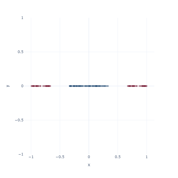
What better place to start an article like this with 1D space? Consider a simple binary classification problem. We have two classes, 0 and 1, represented by three blobs on a number line. The inner blue blob is class 1, and the outer red blobs are class 0.

We know via the universal approximation theorem, that a neural network with at least one hidden layer (of arbitrary dimensionality) can approximate any function.

class Brain(nn.Module):
  """Brain with a single hidden layer."""
  dimensions: int

  @nn.compact
  def __call__(self, inputs):
    out = {}
    x = nn.Dense(self.dimensions, kernel_init=nn.initializers.xavier_uniform())(inputs)
    x = out["activation"] = nn.tanh(x)
    x = nn.Dense(1, name="classifier")(x)
    return x, out

On a number line, the only way to classify these two classes is to find a threshold value. This threshold value is the decision boundary.

We need some boilerplate to train this model. This is a vanilla SGD-based training loop with no fancy regularization or momentum.

def fit(brain: nn.Module, params, x: jnp.ndarray, y: jnp.ndarray):
  """Fit a classification model to the given data."""
  
  @jax.jit
  def train_step(params, x, y, opt_state):
    def loss_fn(params):
      logits, out = brain.apply({"params": params}, x)
      logits = jnp.squeeze(logits)
      loss = optax.sigmoid_binary_cross_entropy(logits, y).mean()
      acc = jnp.mean((logits > 0.5) == y)
      metrics = {"loss": loss, "acc": acc}
      return loss, (metrics, out["activation"])

    (_, (metrics, acts)), grads = jax.value_and_grad(loss_fn, has_aux=True)(params)
    updates, opt_state = tx.update(grads, opt_state, params)
    params = optax.apply_updates(params, updates)

    return params, opt_state, metrics, acts
  
  # Initialize optimizer
  total_steps = 4_000
  tx = optax.sgd(learning_rate=0.01)
  opt_state = tx.init(params)

  # Training loop
  step = 1
  for step in range(1, total_steps + 1):
    params, opt_state, metrics, acts = train_step(params, x, y, opt_state)
    if step % 200 == 0 or step == 1:
      print(f'Step {step}, Loss: {metrics["loss"]:.4f}, Acc: {metrics["acc"]:.4f}')

  return params

To match the 1D world of a number line, we will initialize our model with one dimension. The decision boundary of this neuron will be a point on the number line.

brain = Brain(dimensions=1)
rng, rng_init = jax.random.split(rng)
params = brain.init(rng_init, jnp.zeros_like(x))["params"]
params = fit(brain, params, x, y)

Observe how the activation manifold evolves over time. Since we cannot go anywhere but left or right, the best-accuracy scenario is to push the blue blob as far away from the red blobs as possible, leaving half of red blobs wrongly classified. This gives exactly 75% accuracy.

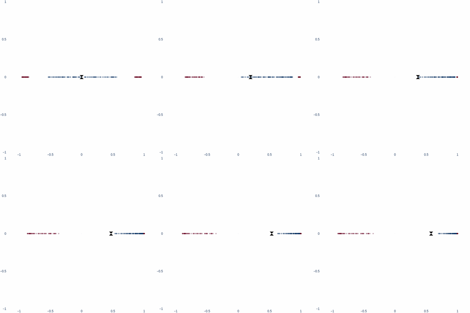
But what if we could think in 2D? Ah, then the problem becomes trivial - we achieve 100% accuracy. Activation space is now a 2D plane, and the decision boundary is a line. Notice how blue cluster is stretched out orthogonally to the red blobs.

Classification in 2D

Let’s redo this exercise, but starting in 2D space. Consider a binary classification problem where the inner blue blob is class 1, and the red ring is class 0.

x, y = datasets.make_circles(n_samples=2048, noise=0.15, factor=0.1)
x = (x - x.mean(axis=0)) / x.std(axis=0)
fig = px.scatter(x=x[:, 0], y=x[:, 1], color=y, color_continuous_scale='RdBu', opacity=0.5)
fig.update_layout(width=600, height=600, coloraxis_showscale=False, template="plotly_white")
fig.show()

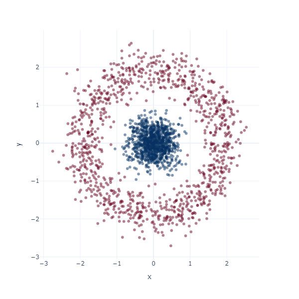
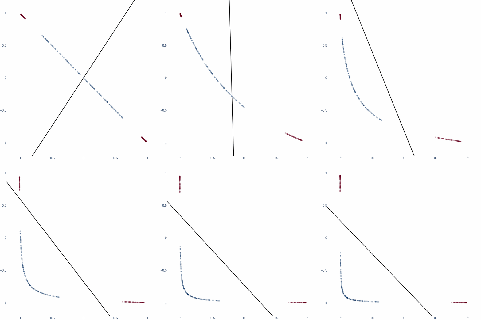
To match the 2D world, we will initialize our model with two dimensions. Visualizing the activation manifold of this 2D model shows the learnt decision boundary. Since activation manifold is 2D, our decision boundary will be a line.

brain = Brain(dimensions=2)
rng, rng_init = jax.random.split(rng)
params = brain.init(rng_init, jnp.zeros_like(x))["params"]
params = fit(brain, params, x, y)

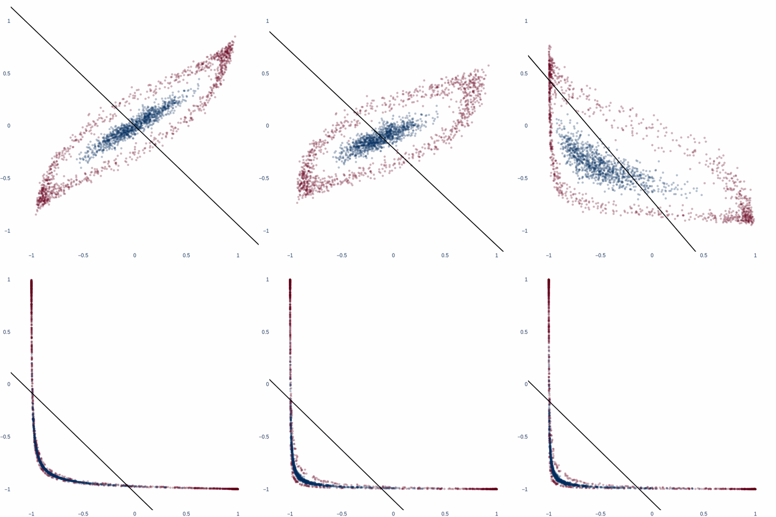
This behavior is similar to the case above where 1D line was expanded to 2D. The entire blue cluster is cornered with red ring stretched out along perpendicular directions. We achieve \(\sim\) 85% accuracy.

But we don’t achieve 100% accuracy on this problem. No line segment can partition these two clusters in 2D space. The outer ring fully covers the inner one. It is mathematically impossible to do so, without using additional dimensions of space. The fact that despite topological limitations, this 2D model crossed \(\sim\) 85% on this dataset tells us how far even a 2D model can twist the data manifold for classification.

Adding the third-dimension

Let’s see what happens when our model is given one extra dimension than the data manifold resides in. Our activation manifold will now be 3D.

brain = Brain(dimensions=3)
rng, rng_init = jax.random.split(rng)
params = brain.init(rng_init, jnp.zeros_like(x))["params"]
params = fit(brain, params, x, y)

The decision boundary is now a plane, which can separate the two classes with \(\sim\) 100% accuracy. This is because the model now stretches the center cluster out across z-axis, and slices a plane orthogonal to it.