Graph Search
Published:
While diving into autograd internals, I had to pause at Topological sort — an important step in backpropagation. Studying it alone felt like buying a single sock. Since I would have to brush up on Depth-First Search anyway (Topological sort’s older sibling), I decided to also toss Breadth-First Search into the cart. After all, who goes shopping for algorithms and leaves with just one?
import random

import matplotlib.pyplot as plt
import numpy as np
from IPython import display
Toy Problem
We will pick a problem of finding a path from the origin (top-left) to the sink (bottom-right) of a randomly generated maze. Our definition of a maze, here, is a mesh of cells with distinct paths that can (or cannot) be traversed. It can be encoded as a graph. There are several ways to encode a graph. We will encode ours as an adjacency matrix, with 1 representing a wall and 0 representing a pathway.
def draw(maze: np.ndarray):
  """Auto-updating plot (note: only if in running in a notebook)"""
  display.clear_output(wait=True)
  plt.figure(figsize=(4, 4))
  plt.axis("off")
  plt.imshow(maze, cmap="plasma_r")
  plt.show()
I will use a simple recusive backtracking algorithm to generate mazes. Here is a goldmine of other algorithms (with beautiful animations) for the curious mind.
def generate_maze(n: int) -> np.ndarray:
  """Generates a random N*N maze using recursive backtracking."""
  # Make `n` odd. Why?
  n -= (n % 2)
  n += 1
  maze = np.ones((n, n), dtype=np.int32)

  # Opening at the top and bottom. We choose these points
  # because we can guarantee that an odd-maze will not have doubly-thick walls.
  maze[0][1] = maze[-1][-2] = 0

  # Direction vectors. Moving by 2 units ensures
  # that we skip over the walls and move from one potential passage to next.
  directions = [(0, 2), (0, -2), (2, 0), (-2, 0)]

  # Choose a random odd coordinate.
  start = (random.randrange(1, n, 2), random.randrange(1, n, 2))
  maze[start] = 0
  stack = [start]

  while stack:
    cy, cx = stack[-1]

    # Get neighbors in a random order.
    random.shuffle(directions)
    found_unvisited_neighbor = False

    for dx, dy in directions:
      nx, ny = cx + dx, cy + dy

      # Check if the candidate cell is not out of bounds and is a wall.
      if (0 <= nx < n and 0 <= ny < n and maze[ny][nx] == 1):
        # Pave thru the wall.
        maze[ny][nx] = 0
        maze[cy + dy // 2][cx + dx // 2] = 0
        # Append new location for paving
        stack.append((ny, nx))
        found_unvisited_neighbor = True
        break

    # Backtrack if all neighbors have been visited.
    if not found_unvisited_neighbor:
      stack.pop()

  return maze

random.seed(42)
maze = generate_maze(50)
draw(maze)
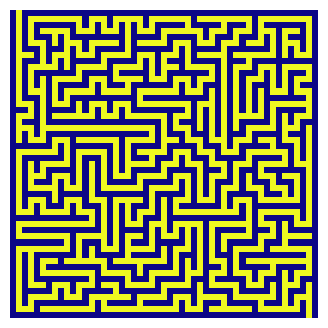
Our goal is to search for a path from the origin (top-left) to sink (bottom-right). During our maze traversal, we are free to explore neighbors one step away.
def get_neighbors(y, x):
  return [
    (y + dy, x + dx)
    for dy, dx in [(1, 0), (-1, 0), (0, 1), (0, -1)]
  ]
Depth-First Search
A key feature of this algorithm is that it exhaustively searches through all possible sub-vertices connected to a given vertex, before backtracking and moving to a different vertex at the same level. It is oblivious to how close it might be to its goal. Other words, even if it is very close to a solution, and then yeets off to a random sub-vertex, it will not return until it has exhaustively searched the dead end.

Tip: Run this in a notebook for an auto-updating plot.
def dfs(graph: np.ndarray,
        start: tuple[int, int] = (0, 1),
        end: tuple[int, int] = (-1, -2),
        visualize: bool = False) -> bool:
  """Checks if a path exists between `start` and `end`."""
  visited = np.zeros_like(graph).astype(np.bool_)

  candidates = [start]
  visited[start] = True

  found = False
  while candidates:
    if visualize: draw(np.where(visited, 0.5, maze))

    # Pick the most recent candidate, i.e. LIFO
    cy, cx = candidates.pop(-1)

    if visited[end]:
      found = True
      break

    for ny, nx in get_neighbors(cy, cx):
      if (
        # within bounds?
        0 <= ny < graph.shape[0] and
        0 <= nx < graph.shape[1] and
        not visited[ny][nx] and
        # not a wall?
        graph[ny][nx] != 1
      ):
        candidates.append((ny, nx))
        visited[ny][nx] = True

  return found

dfs(maze, visualize=True)

DFS search time is proportional to the number of vertices in our adjacency matrix - \(O(N^2)\). The space required to store intermediate states is proportional to the number of vertices (since visited array and candidates stack are the only auxiliary objects in our function), therefore \(O(N^2)\).
Breadth-First Search
A natural modification to DFS could be made on candidate selection. In fact, graph search algorithms like A* and Dijkstra are merely intelligent ways of ‘choosing where to search’. For BFS, instead of going down the rabbit-hole on a single vertex, what if we first explore all vertices available at a given level?
Tip: Run this in a notebook for an auto-updating plot.
def bfs(graph: np.ndarray,
        start: tuple[int, int] = (0, 1),
        end: tuple[int, int] = (-1, -2),
        visualize: bool = False) -> bool:
  """Checks if a path exists between `start` and `end`."""
  visited = np.zeros_like(graph).astype(np.bool_)

  candidates = [start]
  visited[start] = True

  found = False
  while candidates:
    if visualize: draw(np.where(visited, 0.5, maze))

    # Pick candidates in the order they were added, i.e. FIFO.
    # Observe that this is the *only* change from DFS!
    cy, cx = candidates.pop(0)

    if visited[end]:
      found = True
      break

    for ny, nx in get_neighbors(cy, cx):
      if (
        # within bounds?
        0 <= ny < graph.shape[0] and
        0 <= nx < graph.shape[1] and
        not visited[ny][nx] and
        # not a wall?
        graph[ny][nx] != 1
      ):
        candidates.append((ny, nx))
        visited[ny][nx] = True

  return found

bfs(maze, visualize=True)
BFS has the same time and space complexity as DFS in this example - \(O(N^2)\). It also feels parallel. It is because it switches between candidates very quickly - exploring horizontally across each level before exhausting and going to the next level in depth.
Note: We can do a microbenchmark to see that neither of DFS or BFS is relatively faster. This is expected for large, uniformly random mazes. Real world graphs typically carry structure bias towards depth (or width). Hence, your choice of DFS/BFS should be informed by the structure of the graph.
# takes ~1 min
%timeit -n 5 -r 10 dfs(generate_maze(500))
%timeit -n 5 -r 10 bfs(generate_maze(500))
749 ms ± 58.2 ms per loop (mean ± std. dev. of 10 runs, 5 loops each)
778 ms ± 58.8 ms per loop (mean ± std. dev. of 10 runs, 5 loops each)
Topological Sort
Now to the intended goalpost - topological sort. It helps to understand why we need it in the first place. Neural networks are directed acyclic graphs that take a set of input tensor(s), and through multiple operations, return a set of output tensor(s), on which we compute loss, a proxy for how well the network is behaving.
The training objective of neural networks is to minimize this loss by moving along a direction (a.k.a derivative) and [back]propagating this feedback from the loss node to the inputs. Each node in a neural network ‘knows’ how to compute its own derivative only when a gradient signal from the nodes succeeding it is available.
But in a graph with (easily) hundreds of nodes and edges, the autograd engine cannot do a big bang calculation of everything. It must know the exact order of reverse traversal - both for correctness and efficiency of compute.
We will emulate a neural network by generating a web of nodes that are randomly connected to each other between layers. We control this randomness (ten-dollar word is sparsity) using a parameter. Note that if sparsity is too high (say above 0.5), you may end up with unconnected layers. It won’t impact our intent though. I even recommend you experiment with different values to understand how toposort identifies viable orderings.
Bear with me on this boilerplate code to visualize our graph, before we implement toposort(...).
import itertools
import networkx as nx

def generate_mlp(
  layers: list[int],
  sparsity: float = 0.,
  seed: int = 42
) -> tuple[nx.DiGraph, dict]:
  """Generate a layer-wise sparsely connected MLP.

  Args:
    layers: A list of integers denoting nodes in each layer. First and
      last are considered input and output nodes respectively.
    sparsity: A float between [0, 1] representing how sparse the graph
      should be. 0 means no sparsity, i.e. a fully-connected MLP.
    seed: For reproducibility.

  Returns:
    A tuple of nx.DiGraph and options to plot it pretty.
  """
  random.seed(seed)
  num_layers = len(layers)

  # Assign labels to each node.
  input_nodes = [f"$x_{i}$" for i in range(layers[0])]
  hidden_layers = [
    [f"$h^{lyr}_{i}$" for i in range(layers[lyr])]
    for lyr in range(1, num_layers - 1)
  ]
  output_nodes = [f"y{i}" for i in range(layers[-1])]
  layers = [input_nodes, *hidden_layers, output_nodes]

  # Assign nodes.
  G = nx.DiGraph()
  for lyr, nodes in enumerate(layers):
    G.add_nodes_from(nodes, layer=lyr)

  # Assign random edges.
  for left_layer, right_layer in zip(layers[:-1], layers[1:]):
    connections = list(itertools.product(left_layer, right_layer))
    keep_p = 1 - sparsity
    G.add_edges_from(connections[:int(keep_p * len(connections))])

  # Pretty plot.
  pos = nx.multipartite_layout(G, subset_key="layer")
  colors = ["gold"] + ["violet"] * (num_layers - 2) + ["limegreen"]
  options = {
    "node_color": [colors[data["layer"]] for node, data in G.nodes(data=True)],
    "with_labels": True,
    "node_size": 1000,
    "pos": pos,
  }

  return G, options

G, options = generate_mlp([3, 4, 6, 4, 6, 1], sparsity=0.5)
nx.draw(G, **options)
plt.show()
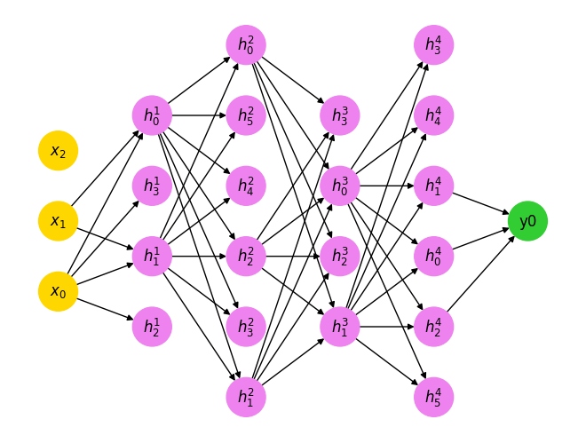
The only important observation is that not all nodes may influence the terminal loss node (indexed as \(y_i\)) in this example. Our sorting algorithm should identify this.
In other words, for a root node loss, the autograd engine needs a list of all dependencies to loss all the way to input tensor(s), in the order they impact it. This is like searching along the depth from the loss node (did it click in your mind?). We will use toposort to find these orderings from a given root node to the stopping points on the graph (i.e. nodes with no more ancestors) via depth-first search.
def toposort(G: nx.DiGraph, root: str):
  """Returns a topological ordering from `root` on the graph `G`."""
  visited = set()
  order = []

  def _dfs(node):
    if node not in visited:
      visited.add(node)
      # If the node has ancestors, DFS along each.
      for parent in G.predecessors(node):
        _dfs(parent)

      # Once all ancestors have been evaluated,
      # add the node to the topological order.
      order.append(node)

  # Start searching for stopping points from the root.
  _dfs(root)

  # Because we start from the root node.
  order.reverse()
  return order

order = toposort(G, 'y0')
order
['y0',
 '$h^4_2$',
 '$h^4_1$',
 '$h^4_0$',
 '$h^3_1$',
 '$h^3_0$',
 '$h^2_2$',
 '$h^2_1$',
 '$h^2_0$',
 '$h^1_1$',
 '$h^1_0$',
 '$x_1$',
 '$x_0$']
Modulo the ugly \(\LaTeX\) formatting, We can see that toposort returns an ordering from output node(s) to input node(s) whenever there is a path connecting them.
Let’s draw these backward edges.
def draw_backward_traversal(G: nx.DiGraph, order: list[str]):
  """Plots the reverse traversal of nodes given in `order` on the graph `G`."""
  edges = []
  for node in order:
    # Point incident edges backwards
    incident_edges = G.in_edges(node)
    incident_edges = [e[::-1] for e in incident_edges]
    edges.extend(incident_edges)

  nx.draw(G, edgelist=edges, edge_color="red", **options)
  plt.show()

draw_backward_traversal(G, order)
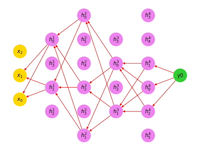
See? The topological ordering automatically ignores nodes (even inputs) that do not influence the output.
N.B: This is a possibly unconventional example of sparsely-connected MLPs. In practice, MLPs are trained fully-connected. I should have used a better terminology, in that these graph nodes are arbitrary functions themselves. But I am sure it gets the idea across.
We knew it all along, didn’t we?
This exercise taught me that algorithms of this class are actually straightforward to understand if you have a view of the entire graph and you know the objective. The challenge lies in expressing your computation in a way computers can understand. Specifically:
- How can you identify a sub-problem that can be recursed/iterated over.
- How and when to recurse/iterate over that subproblem, and
- How to book-keep states efficiently.
We take for granted how much our brain does this in a diffused manner. Luckily, with frontier language models getting better, ‘talking’ with computers will get easier.
I hoped to cover Dijkstra and A* as well, given how they add a sprinkle of intelligence (read heuristics) to solve certain classes of graph problems faster. That will be a different article for now.